本科毕业设计(论文)
外文翻译
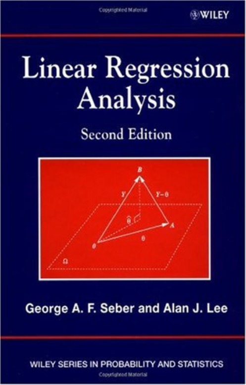
Linear Regression Analysis
作者:George A.F.Seber ,Alan J.Lee
国籍:America
出处: George A.F.Seber .Linear Regression Analysis .35-36,97-98,391-394
原文正文:
Let Y be a random variable that fluctuates about an unknown parameter that is, , where c is the fluctuation or error. For example, c may be a 'natural' fluctuation inherent in the experiment which gives rise to , or it may represent the error in measuring , so that is the true response and Y is the observed response. As noted in Chapter 1, our focus is on linear models, so we assume that can be expressed in the form
.
where the explanatory variables are known constants (e.g., experimental variables that are controlled by the experimenter and are measured with negligible error), and the () are unknown parameters to be estimated. If the are varied and n values, ,...,, of Y are observed, then
where is the ith value of . Writing these n equations in matrix form, we have
,
Or
where . The matrix X will be called the regression matrix, and the are generally chosen so that the columns of X are linearly independent; that is, X has rank p, and we say that X has full rank. However, in some experimental design situations, the elements of X are chosen to be 0 or 1, and the columns of X may be linearly dependent. In this case X is commonly called the design matrix, and we say that X has less than full rank.
It has been the custom in the past to call the xis the independent variables and Y the dependent variable. However, this terminology is confusing, so we follow the more contemporary usage as in Chapter 1 and refer to as a explanatory variable or regressor and as the response variable.
As we mentioned in Chapter 1, (3.1) is a very general model. For example, setting and , we have the polynomial model
Again,
is also a special case. The essential aspect of (3.1) is that it is linear in the unknown parameters ; for this reason it is called a linear model. In contrast,
is a nonlinear model, being nonlinear in .
Before considering the problem of estimating , we note that all the theory in this and subsequent chapters is developed for the model (3.2), where is not necessarily constrained to be unity. In the case where , the reader may question the use of a notation in which i runs from to rather than to . However, since the major application of the theory is to the case , it is convenient to 'separate' from the other rsquo;s right from the outset. We shall assume the latter case until stated otherwise.
One method of obtaining an estimate of is the method of least squares. This method consists of minimizing with respect to that is, setting, we minimize subject to , where is the column space of (). This is obvious geometrically, and it is readily proved algebraically as follows.
Hypothesis Testing:
In this chapter we develop a procedure for testing a linear hypothesis for a linear regression model. To motivate the general theory given below, we consider several examples.
From (1.1) we have the model:
representing the force of gravity between two bodies distance apart. Setting and , we have the usual linear model , where an error term has been added to allow for uncontrolled fluctuations in the experiment. The inverse square law states that beta; = 2, and we can test this by taking n pairs of observationsand seeing if the least squares line has a slope close enough to 2, given the variability in the data.
Testing whether a particular in a regression model takes a value other than zero is not common and generally arises in models constructed from some underlying theory rather than from empirical considerations.
EXAMPLE 4.2 From (1.2) we have the following model for comparing two straight lines:
,
where, , , and · To test whether the two lines have the same slope, we test; while to test whether the two lines are identical, we test .. Here we are interested in testing whether certain prespecified are zero.
EXAMPLE4.3 Suppose that we have the general linear model :
G:
Or When is large We will usually be interested in considering whether we can set some of the equal to zero. This is the problem of model selection discussed in Chapter 12. If we test the hypothesis , then our model becomes
H:
Or Here consists of the first r columns of .
Prediction and Model Selection:
The aim of regression analysis is to discover the relationships, if any, between the response and the explanatory variables . Ultimately, we may wish to use these relationships to make predictions about Y based on observing . Alternatively, we may use the fitted model to better understand how particular variables are related to the response. In both cases, we need to choose a tentative model to fit to the data. Having fitted the model, we need to assess how well the model fits, and if necessary, modify the model to improve the fit, using the methods of Chapter 10. We can then use the fitted model to make predictions.
An important part of this process is to decide which variables to include in the model and how to construct a predictor from the variables available. In the first part of this book we assumed that the set of variables was given. In this chapter we assume that a large number K of potential explanatory variables are available. We shall discuss ways of selecting which variables to include in order to get a good model, and how to use the available variables to construct a good predictor.
If the main aim of the analysis is to m
剩余内容已隐藏,支付完成后下载完整资料


英语原文共 583 页,剩余内容已隐藏,支付完成后下载完整资料
资料编号:[276761],资料为PDF文档或Word文档,PDF文档可免费转换为Word
以上是毕业论文外文翻译,课题毕业论文、任务书、文献综述、开题报告、程序设计、图纸设计等资料可联系客服协助查找。


